The Department of Biology at Lund University maintain a record of 3D models or ‘meshes’ of biological specimen. These records are used for investigating how the species diverge, adapt, and evolve on a microscopic scale in response to different environmental factors. The methods for producing these models often involves scanning the specimen with Computer Tomography (CT Scan) and then extracting the surface contour of the resulting volume with a certain (or several) isovalues. The second part, namely producing the mesh from the volumetric data, are readily available in a plethora of different software solutions, and they have their different benefits and drawbacks.

There are two common problems to overcome in the second part of the production pipeline described above, removing noise and computationally managing large amounts of data.

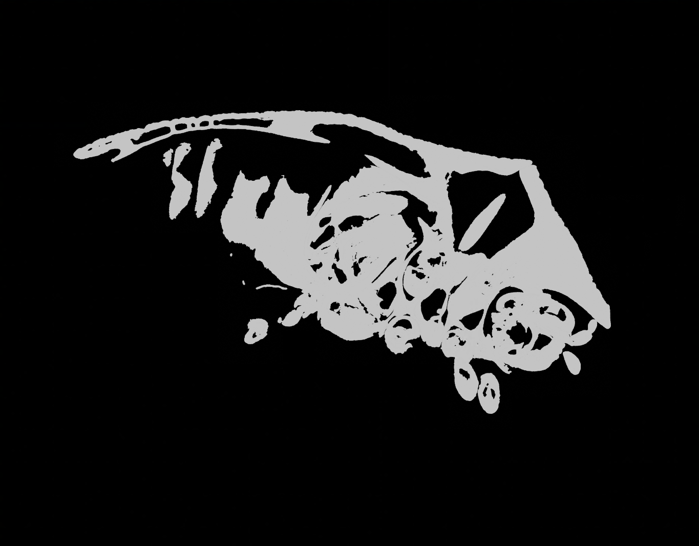
Many volumetric scanning techniques will invariably introduce noise to the “empty space” of the data set. This is not a problem if the range of the noise does not contain the isovalue for the surface extraction, as then the algorithm would simply just not draw faces for those noise values. However, when the isovalue is within the noise range, then small noisy components will be generated in the surface extraction. These noise components detract from the clarity of the data set and bloats the file’s size in terms of memory and processing steps.

With improved scanning machineries, the fidelity of the data set is also improved. In 3D environments, the increase in general fidelity leads to a cubic increase to the amount of data that needs to be processed. Noise bloating the data set is also a contributing issue to the problem of memory management. The increased amount of data becomes very much prohibitive to conventional computational systems that are usually available to researchers. While using supercomputers is technically a viable option, options that do not involve supercomputing should typically be exhausted first. These methods usually involve optimisation and smarter use of memory and processing, as to not overwhelm the processing unit.

This project deals mainly with providing user-friendly methods for facilitating the production pipeline for the researchers producing 3D models from CT scans, while also dealing with noise and increased sizes of data sets.

Source(s) used: Giuseppe Bianco, Maja Tarka

Project Details

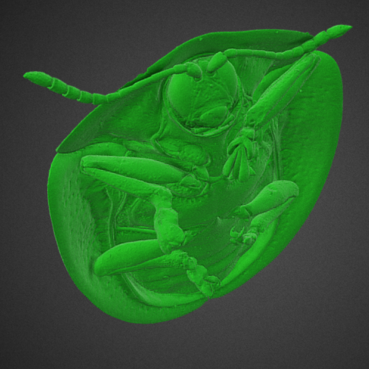
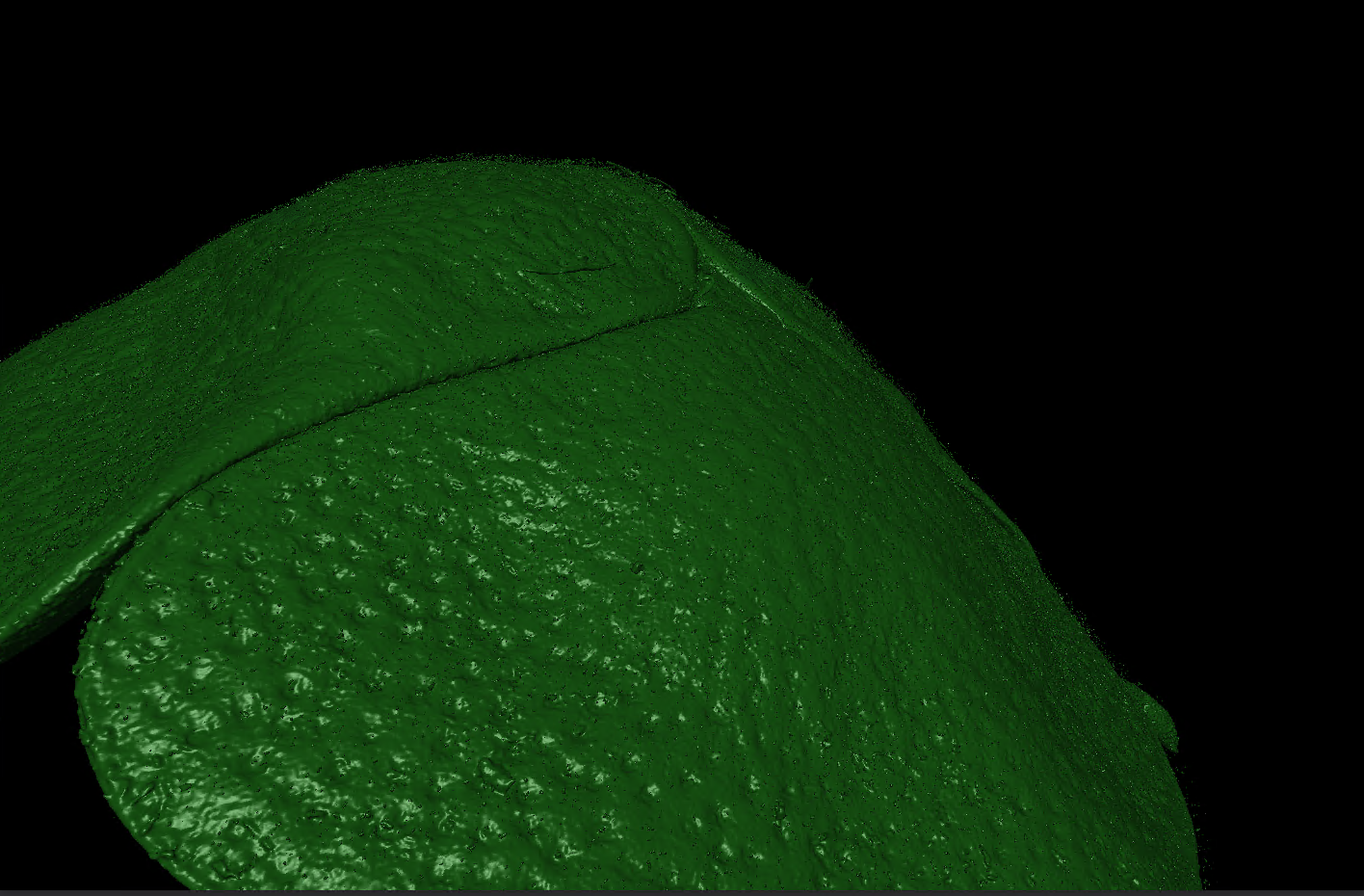
The Green Tortoise Beetle ‘Cassida Viridis’ is used in Maja Tarka’s research group as a model system for studying microevolution and adaptation in wild insect populations (Maja Tarka — Lund University). Because of this, the data representing such a specimen became the working volume dataset in this InfraVis project for trying out the pipeline on. The raw dataset is ~10 GB and its dimensions are ~2500x2000x1000, which results in about 5 billion points in a scalar, uniform grid. The reader may note that the beetle is missing two legs; yes, it lost two legs before or during the process of it being scanned.

The first part of the project was defining a production pipeline that was easily accessible for researchers in any domain that would want to produce their own meshes from a CT scan. While most would know a basic amount of programming, writing code or command line arguments would likely lead to a low retention of the learned procedures. A more visual way, that is already set up, with only changing a few parameters being necessary between different tasks, was the way to go in our minds. This pipeline should also implicitly support large workloads, and should fully utilise the resources available to the processing system, meaning arbitrary CPU, Memory, or GPU limitations from a software solution would not be ideal.

A visualization toolkit, Inviwo, was suggested, mainly from the InfraVis team’s own familiarity with the tool and the Open Source access to it. It uses a visual, graph-based layout for each workspace or ‘program’, where data tends to “flow down” the graph. It is also built with scientific visualization in mind, so fully using the system’s resources is a set priority by its developers. The idea is not that the users in this project will build their workspace themselves, but at least know how to edit the parameters of it and make small changes to it. If they get even more onboard with Inviwo, then that is just a bonus. The software is either installed directly with a downloadable .exe from their website or build from source from their GitHub repository. Both versions are free of charge, while the former is easier, but without possibility for modules or writing/changing any processors; the latter is more complicated, but with additional freedom with adding modules or altering the code of the program itself. For this specific project, the already built installation was determined to be sufficient, as it had all the necessary features.

The way one builds a visualization pipeline in Inviwo involves importing some kind of input, using input or source nodes; processing that data, using intermediary nodes; and then presenting that directly on a canvas or as a file export, using output or sink nodes. By designing these nodes for different scenarios and formats of data, the developers enables the user to very easily set up many different kind of rendering pipelines in Inviwo, without getting into the gritty details of actually writing code.

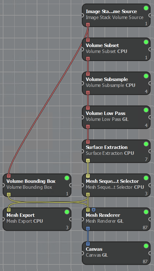
To explain in more detail what the InfraVis users needed this pipeline to do, it needs to be stated first what is the input and what is the output. The input is a volume in the form of a stack of .tif images representing each of the CT slices, and the output is a 3D object representing the surface of the beetle.

The source processor ‘Image Stack Volume Source’ deals with constructing a cohesive volume from a directory of slice images. After the volume has been loaded, it can then be trimmed to cut out irrelevant empty space outside the bounding box of the interesting data, and then subsampled to a desired degree of reducing the data. To deal with the noise, a low pass filter removes many of the high-frequency noise in the volume, without any drastic changes to the interesting parts of the data.

With the volume prepared with different pre-processing options, creating an actual 3D object from the volume is most commonly done with a surface extraction. It builds faces for each cell in the volume that represent a certain spatial value, that is aptly named isovalue. It is meant to draw faces in the volume everywhere this static value exists, which will involve some interpolation in a structured grid. The isovalue that was most accurately representing the surface of the object was determined to be 7226, in this case.

With the 3D object extracted from the volume, it could now be rendered in Inviwo’s own renderer or exported as a stereolithographic (.stl) or Wavefront (.obj) object, to then be further processed in another software or used directly.

With the pipeline set up and working, it is usually not working, unless the user allows some concessions to be made. The unaltered volume simply produces a way too large mesh for most systems to handle. There are three simple ways to go about dealing with this in Inviwo: Subsetting, subsampling, and low pass filtering.

Subsetting reduces to problem to a subsection of the original volume, which will reduce the problem size accordingly. The issue with this approach is that if you want the whole thing, you need some process afterwards to glue these subsections afterwards, which would require additional work and also simply just create the same issue as before. Subsetting the volume is at the very least good enough to exclude the empty, noisy regions directly outside the immediate bounding box of the interesting part.

Subsampling reduces the problem size by simply ignoring every cell, other than every nth cell, in any of the cardinal directions. E.g. a subsample of 2x2x2 effectively removes 7/8 of all cells , by removing ever second cell in each direction. This process preserves the wholeness of the volume, but sacrifices detail. It is often an effective trade-off worth doing to get some output, but it should be done as little as is necessary to this end.

The low pass filtering is a method that is essentially a gaussian blur. It effectively evens out high-frequency differences in the volume, while maintaining the overall geometry, as actual geometry tends to not differ too much. While it is quite effective at eliminating noise, one should always bear in mind that it does alter the data in ways that may obfuscate or even misconstrue the underlying truths one wants to observe. It is best to avoid low pass filtering whenever possible, and to minimise its influence if it isn’t possible to avoid.

Once a mesh is produced, any lingering noise is easily removed in any 3D modelling software by inverting the selection of the largest component in the entire mesh, and deleting the inverted selection. This assumes of course that the mesh can be loaded in this scenario, which was not always be the case in this project. We found that doing 2x2x2 subsampling, with a low pass filter kernel of size 3 afterwards, made a reasonably sized mesh to work with in post-processing, with only these three options to go for. Then, the mesh could be decimated to reduce the amount of faces with a factor that made most sense for the end use, which resulted in the listing on Sketchfab, which can be viewed below.

Green Tortoise Beetle (Cassida viridis) by 3D Lab – Department of Biology – Lund University on Sketchfab

This marks the end of the project from the experience of the users, but there was more work to be done to reduce the issues introduced by the standard methods, that is further explained below.

Bonus Project

This next part goes beyond what the users initially asked for, but was explored just for the case of future, similar projects. Because of the sheer size of the dataset, it was prohibitively difficult to process it in different programs. Because of this, we thought out ways to, in the end, reduce the amount of faces that needed removal in the 3D modelling programs. The result was two methods that would work in theory, but remained up until now untested in practice. The first method involves more accurately eliminating noise that are clearly, in terms of distance to the object of interest, in the “empty space”. The second method involves processing the resulting ungainly large mesh in a simple script that doesn’t need to load the entirety of the mesh at once.

Eliminating Noise Pre-render

Eliminating the noise before even creating the mesh would involve ‘masking’ the volume before it was used. We would need to set all the ’empty space’ pixels to ‘0’ to eliminate all the noise. Since the volume consists of an image stack, this can in theory be done in any image editing program, manually masking each slice as needed. In practice however, this would be many unnecessary laborious hours. How could we automatically mask each slice in a semi-supervised manner? The answer is simple when you think about it: Use the resulting mesh to mask the original volume. Remember that subsampling the mesh preserves the overall geometry of the model, but removes the detail, so we could generate a low-fidelity mesh with subsampling, remove the noise from it, ‘fatten’ the mesh a little to compensate for a slight loss of detail and geometry, then virtually ‘slice’ it, and then use a binary representation of these slices to mask the original slices.

The virtual tomography was done in Blender and the masking was done with ImageJ. The result was not particularly effective in terms of magnitude; as the memory reduction was only 40-60 % for this dataset, which was still prohibitively large to process after. If such a reduction does however bring your mesh below the threshold of what you can work with in any other case, the method may be worth it. The two drawbacks of this method was that the virtual tomography took a few days to finish and that it requires intermediate proficiency with modelling programs.

Processing the Object File

The other method recognises the ever true notion that the mesh file can be edited to keep the relevant parts and discard the rest, even in a simple file-processing script in Python. What is done in Blender to remove noise can also be done in this script. The issue with many modelling programs is that it loads the entire mesh to memory when working with it, with all the surplus bloated extra information that is important for editing the mesh, yes, but not for this simple process. Keeping the data ‘on disc’ while only loading the memory with the relevant details we choose ourselves, this should relieve the strain on the working memory.

The massive mesh file was imported from Inviwo as a Wavefront (.obj) object. Going through the structure of Wavefront objects produced in Inviwo, it has entries for vertices, normals, UVs, and faces. Only vertices and faces are important here, but normals are less than obvious to reconstruct later. UVs can safely be discarded here, though. Other than that, the script needed to replicate the work flow in Blender; find the largest component(s), and then delete all other components not part of them. The script is correct, for sure, but for the sheer size of the mesh, completely untenable to process the mesh. There were over 67 million vertices in the non-reduced mesh, and one night of processing only went through the first ~1.5 million. Maybe if the process could be optimised in another programming language or just through the method itself, would it be tenable, but at this point, time was running out.